The Small Phylogenetic Trees website is mainly a repository of algebraic information of
different evolutionary models based on trees with a small number or leaves. Here, small means at most five
leaves. This website is meant as a companion of Chapter 15: Catalog of Small Trees in the book
"Algebraic Statistics for Computational Biology", Pachter and Sturmfels (editors), Cambridge University Press.
One of the most important features is the introduction of a unified notation across all trees and models to describe all tree properties.
The goal of specifying a notation is to uniquely specify all components of an evolutionary model on a tree just from a given picture
of the tree. We hope that this notation will make communication among researchers in this area easier by avoiding the tedious work of translating different
notations to be able to understand each other.
In the book "Inferring Phylogenies", Felsenstein writes: "... invariants are worth attention, not for what they do for us now, but what they might lead in the future...".
It is our hope for this website to bring the future even closer. Feel free to check some of the applications of this website at the end of this page.
If you know of more applications where this website might be useful please let us know.
The following is a guideline to the different parts of this website.
- The trees
- The trees in this website are divided in two categories: rooted trees and unrooted trees. Currently all rooted trees are assumed to have
uniform root distribution but in the future we will also include tree models with arbitrary root distribution. Furthermore, the Molecular Clock condition
is assumed in all rooted trees. Unrooted trees stand for rooted trees with uniform root distribution and no molecular clock assumption. It is a fact that for this type
of trees the root can be placed anywhere in the tree; thus justifying the notion of unrooted tree. One more reason to consider unrooted trees is that (the invariants associated to)
any rooted tree with unknown root distribution is equivalent to (the invariants associated to) an unrooted tree with one more leaf directly attached to the root of the original tree.
A future project involves describing trees with unknown root distribution as well.
- The models
- Currently, there are only four evolutionary models discussed in this website: the Neyman 2-state model (N71), the Jukes-Cantor DNA model (JC69), the
Kimura 2-parameter model (K80), and the Kimura 3-parameter model (K81). The Felsenstein hierarchy of evolutionary models gives a brief summary of these models.
The N71 model is also referred as the Binary Symmetric model, this model assumes that the data is binary. In the future, we would like to include more models in this website.
- The Molecular Clock assumption
- The standard interpretation of the MC assumption is that certain sums of evolutionary times are equal
to each other. This is equivalent to saying that certain products of transition matrices should be the same. More precisely,
the molecular clock (MC) assumption for a rooted tree T states
that for each subtree and each path from the
root of that subtree to any leaf i, the products of the transition
matrices corresponding to the edges of the path are identical. As the edges
are visited along the path, the matrices are multiplied left to
right.
This is justified because all transition matrices in the group-based models actually commute with each
other.
- The substitution matrices
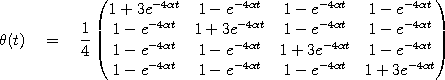
- In computational biology literature it is common to associate to each edge in the tree
a substitution matrix that depends on two parameters t and
 . For example, in the Jukes-Cantor model
the substitution matrix is given by
Since the probabilities in the substitution matrix
. For example, in the Jukes-Cantor model
the substitution matrix is given by
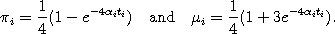
Since the probabilities in the substitution matrix  do not depend polynomially on the parameters and t, it is customary to
make the following change of variables in the space of
parameters. Instead of using
do not depend polynomially on the parameters and t, it is customary to
make the following change of variables in the space of
parameters. Instead of using  and ti, two new parameters
are introduced
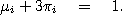
These parameters satisfy the linear constraint
These parameters are the entries in the
substitution matrix used to compute the parameterization of the model.
and ti, two new parameters
are introduced
These parameters satisfy the linear constraint
These parameters are the entries in the
substitution matrix used to compute the parameterization of the model.
- The parameterizations
- For each model we describe two parameterizations. One parameterization given by the joint probabilities of all leaf colorations of the tree, Each probability is a polynomial
in the parameters of the model. Two of these probabilities are equivalent if their defining polynomials are identical.
This divides the joint probabilities into equivalent classes. For each class i there is an indeterminate pi which denotes the sum of the probabilities in the class.
The second parameterization, called Fourier parameterization, results from expressing the first parameterization in terms of an alternative coordinate system,
where the change of basis is given by the Fourier transform. The Fourier parameterization has the amazing property that all coordinates are actually (Laurent) monomials, and thus much easier to work with.
Similarly, we split the coordinates of this parameterization into classes. For each class j there is an indeterminate qj that denotes the average of the Fourier coordinates in the class.
- The Fourier transforms
- The Fourier transform provides a linear change of coordinates in the parameter space of the model and it simultaneously gives a linear change of coordinates in the probability space.
The Fourier transform can be compressed into a linear transformation from the indeterminates pi to the indeterminates qj. This transformation is called specialized Fourier transform. In general, this matrix is not
square and hence its inverse is in general only a right-inverse.
- The invariants
- All statistical models of evolution in this website are algebraic varieties in the space of joint probability distributions on the leaf colorations of the corresponding tree.
The phylogenetic invariants of a model are the polynomials which vanish on the variety. Furthermore, the invariants of every model in this website form a toric ideal in the Fourier coordinates.
We record a minimal generating set for the ideal generated by the invariants. Such a generating set should be useful in some applications, for example, when trying to evaluate all invariants of a model at a specific probability
distribution. Clearly, the least number of polynomials to be evaluated the better. We also record a reduced degree reversed lexicographic Gröbner basis for the ideal of invariants. In computational algebra, a Gröbner basis
is the best way to represent a given ideal, because it allows to compute many numerical invariants associated to the ideal.
- The software
- Most computations were done in the computer algebra systems: Maple and Singular. The invariants were computed using 4ti2;
nevertheless, subsequent invariant computations will be done using a package being written in Perl that implements the methods developed by Sullivant and Sturmfels to compute this invariants.
We have tried to keep all data in this website system-free or at least system-friendly. But for each model, we have included both a Maple and a Singular file that contains all the information associated to the model system-ready.
We have written many Singular libraries with procedures to work with phylogenetic tree models and other statistical models. We are in the process of including them into the main Singular distribution. Most documentation for this libraries
has not been written yet, thus we have not included them in this website yet. Nevertheless, some parts of them have been linked in the
Algebraic Statistics for Computational Biology website.
Please note that the Singular files use a couple of procedures included in the Singular file suma.sing. The portion of the file that uses those procedures has been commented out by default.
- The files
- All files have been saved as plain text files and can be opened on any text editor. All files larger than 500 Kbytes have been compressed using the command bzip2. To
unzip them in Linux, Unix, or Mac os X use the command 'bunzip2' or 'bzip2 -d'. In windows, there are several (freeware) packages that can unzip these files like 7-Zip or WinBZip2.
But you can also download the bzip2 program for windows from the bzip website.
- The applications
- In Chapter 15 of the "Algebraic Statistics for Computational Biology" book it is reported an application of the
phylogenetic invariants to infer tree topologies from data. Actually, [Cavender and Felsenstein, 1987] and [Lake, 1987] introduced phylogenetic invariants as an algebraic tool for reconstructing evolutionary trees
from biological sequence data.
In Chapter 18 the authors report about an application of these invariants and exact methods to compute the ML of a model from the ML equations to reconstruct phylogenetic trees. These authors use a method called Generalized Neighbor-Joining introduced in the paper
"Beyond pairwise distances:
neighbor joining with phylogenetic diversity estimates" by Levy, Pachter, and Yoshida.
One simple but powerful application is the use of the indeterminates pi as sufficient statistics for a given model. These allows to compress
much further some given biological sequence data. The gain in speed for any algorithm that processes this type of data using these models could be significant.